how to find upper and lower bounds

The Lower and Upper Bound Theory provides a way to find the lowest complexity algorithm to solve a problem. Before understanding the theory, first lets have a brief look on what actually Lower and Upper bounds are.

Lower Bound –
Let L(n) be the running time of an algorithm A(say), then g(n) is the Lower Bound of A if there exist two constants C and N such that L(n) >= C*g(n) for n > N. Lower bound of an algorithm is shown by the asymptotic notation called Big Omega (or just Omega).
Upper Bound –
Let U(n) be the running time of an algorithm A(say), then g(n) is the Upper Bound of A if there exist two constants C and N such that U(n) <= C*g(n) for n > N. Upper bound of an algorithm is shown by the asymptotic notation called Big Oh(O) (or just Oh).

1. Lower Bound Theory:
According to the lower bound theory, for a lower bound L(n) of an algorithm, it is not possible to have any other algorithm (for a common problem) whose time complexity is less than L(n) for random input. Also every algorithm must take at least L(n) time in worst case. Note that L(n) here is the minimum of all the possible algorithm, of maximum complexity.
The Lower Bound is a very important for any algorithm. Once we calculated it, then we can compare it with the actual complexity of the algorithm and if their order are same then we can declare our algorithm as optimal. So in this section we will be discussing about techniques for finding the lower bound of an algorithm.

Attention reader! Don't stop learning now. Get hold of all the important DSA concepts with the DSA Self Paced Course at a student-friendly price and become industry ready. To complete your preparation from learning a language to DS Algo and many more, please refer Complete Interview Preparation Course .

In case you wish to attend live classes with experts, please refer DSA Live Classes for Working Professionals and Competitive Programming Live for Students.

Note that our main motive is to get an optimal algorithm, which is the one having its Upper Bound Same as its Lower Bound (U(n)=L(n)). Merge Sort is a common example of an optimal algorithm.

Trivial Lower Bound –
It is the easiest method to find the lower bound. The Lower bounds which can be easily observed on the basis of the number of input taken and the number of output produces are called Trivial Lower Bound.

Example: Multiplication of n x n matrix, where,

          Input: For 2 matrix we will have 2n²          inputs          Output: 1 matrix of order n x n, i.e.,  n²          outputs

In the above example its easily predictable that the lower bound is O(n²).

Computational Model –
The method is for all those algorithms that are comparison based. For example in sorting we have to compare the elements of the list among themselves and then sort them accordingly. Similar is the case with searching and thus we can implement the same in this case. Now we will look at some examples to understand its usage.

Ordered Searching –
It is a type of searching in which the list is already sorted.
Example-1: Linear search
Explanation –
In linear search we compare the key with first element if it does not match we compare with second element and so on till we check against the nth element. Else we will end up with a failure.

Example-2: Binary search
Explanation –
In binary search, we check the middle element against the key, if it is greater we search the first half else we check the second half and repeat the same process.
The diagram below there is an illustration of binary search in an array consisting of 4 elements

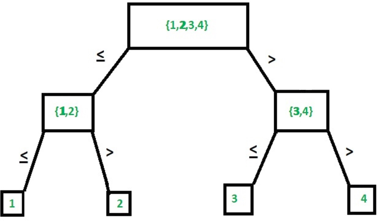
Calculating the lower bound: The max no of comparisons are n. Let there be k levels in the tree.

No. of nodes will be 2^k-1
The upper bound of no of nodes in any comparison based search of an element in list of size n will be n as there are maximum of n comparisons in worst case scenario 2^k-1
Each level will take 1 comparison thus no. of comparisons k≥|log₂n|

Thus the lower bound of any comparison based search from a list of n elements cannot be less than log(n). Therefore we can say that Binary Search is optimal as its complexity is Θ(log n).

Sorting –
The diagram below is an example of tree formed in sorting combinations with 3 elements.

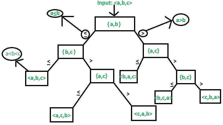
Example – For n elements, finding lower bound using computation model.

Explanation –
For n elements we have a total on n! combinations (leaf nodes). (Refer the diagram the total combinations are 3! or 6) also it is clear that the tree formed is a binary tree. Each level in the diagram indicates a comparison. Let there be k levels => 2^k is the total number of leaf nodes in a full binary tree thus in this case we have n!≤2^k.

As the k in the above example is the no of comparisons thus by computational model lower bound = k.

Now we can say that,          n!≤2^T(n)                    Thus,  T(n)>|log n!|  => n!<=nⁿ          Thus, log n!<=log nⁿ          Taking ceiling function on both sides, we get |^-log n^n-|>=|^-log n!^-| Thus complexity becomes Θ(lognⁿ) or Θ(nlogn)

Using Lower bond theory to solve the algebraic problem:

Straight Line Program –
The type of programs build without any loops or control structures is called Straight Line Program. For example,

C

Sum(a, b)

{

c:= a+b;

return c;

}

Algebraic Problem –
Problems related to algebra like solving equations inequalities etc., comes under algebraic problems. For example, solving equation ax²+bx+c with simple programming.

C

Algo_Sol(a, b, c, x)

{

v:=a*x;

v:=v+b;

v:=v*x;

ans:=v+c;

return ans;

}

Complexity for solving here is 4 (excluding the returning).
The above example shows us a simple way to solve an equation for 2 degree polynomial i.e., 4 thus for n^th degree polynomial we will have complexity of O(n²).

Let us demonstrate via an algorithm.

Example: x+a₀ is a polynomial of degree n.

C

pow (x, n)

{

p := 1;

for i:=1 to n

p := p*x;

return p;

}

polynomial(A, x, n)

{

int p, v:=0;

for i := 0 to n

v := v + A[i]* pow (x, i);

return v;

}

Loop within a loop => complexity = O(n²);
Now to find an optimal algorithm we need to find the lower bound here (as per lower bound theory). As per Lower Bound Theory, The optimal algorithm to solve the above problem is the one having complexity O(n). Lets prove this theorem using lower bounds.

Theorem: To prove that optimal algo of solving a n degree polynomial is O(n)
Proof: The best solution for reducing the algo is to make this problem less complex by dividing the polynomial into several straight line problems.

=> a_nxⁿ+a_n-1x^n-1+a_n-2x^n-2+...+a₁x+a₀          can be written as,  ((..(a_nx+a_n-1)x+..+a₂)x+a₁)x+a₀          Now, algorithm will be as, v=0 v=v+a_n          v=v*x v=v+a_n-1          v=v*x ... v=v+a₁          v=v*x v=v+a₀

C

polynomial(A, x, n)

{

int p, v=0;

for i = n to 0

v = (v + A[i])*x;

return v;

}

Clearly, the complexity of this code is O(n). This way of solving such equations is called Horner's method. Here is where lower bound theory works and give the optimum algorithm's complexity as O(n).
2. Upper Bound Theory:
According to the upper bound theory, for an upper bound U(n) of an algorithm, we can always solve the problem in at most U(n) time.Time taken by a known algorithm to solve a problem with worse case input gives us the upper bound.